Friday 24 September 2021

CanSat Competion 2020-2021: The Launch

On Friday the 16th of September the launch of ESERO CanSat competition 2020-2021 took place. The original launch had been postponed due to covid-19 restrictions, but thankfully  measures were relaxed and the launch became possible. Our team, the Canservationists, from the British School in the Netherlands, was there.

Although the progress during covid was challenging, in addition to technical challenges we faced (for which information and how we tackled them can be found here and here), we managed to accomplish our mission (final progress report and a very nice video can be found here) and earn the 3rd place at national level.

Our CanSat was in the first launch window (many thanks to DARE TU Delft team for the great rockets and supporting the launches) and was launched around midday along with three other CanSats.

 
Vaggelis putting our CanSat into the rocket

We were happy to see that our CanSat not only survived the landing, but we were also able to collect all our intended measurements. 

What went well: 

- Not only did we get our CanSat back in one piece, but it was fully intact as well. This showed that its construction was extremely robust and that our hand-made parachute worked!

- As said, all the sensors worked and collected all the intended measurements (humidity, pressure, temperature, CO2, Total volatile organic compounds - TVOC). Our Arduino code that made all this possible can be found here. You will find the results below. 

- The chosen battery was good enough to support the whole process, irrespective of having the CanSat 'on' for quite some time before the launch (see results below). 

What worked, but could be improved:

- Our GPS sensor could not update the position fast enough to cope with the extremely fast moves during the launch. This also affected the enabling of our buzzer during landing which was supposed to be triggered by the GPS sensor. Fortunately, we were also measuring the altitude via pressure sensor which, despite a systematic error of some tens of metres, worked very well. 

- We managed to receive some of the measurements through telemetry, but not all the time. Given that we cannot change the CanSat itself very much (due to its size and power limitations), a more powerful ground station and a ground antenna with more gain than the Yagi we used may help.

Analysing the results, first we had to identify the data that corresponded to the launch (and especially the landing). To this end, we used the altitude. In the figure below, the spike clearly indicates when the launch took place. 

As we can see, our CanSat was 'on' for more than an hour until eventually was launched. 

In the diagram below we can see that the GNSS (GPS) sensor could not cope with the abrupt changes (its measurements seem very 'digital').

In the diagram below the temperature measurements are depicted. The abrupt change during the launch is evident. Moreover, the measured temperature decreases as the CanSat goes down, instead of increasing as we normally would expect. This is due to the influence of the rocket during launch.   

In the figure below, the CO2 measurements are depicted. No concrete conclusion can be drawn, except from the fact that CO2 concentration increases significantly near the ground.

This is also the case with the TVOC measurements where, again, values increase rapidly near the ground.

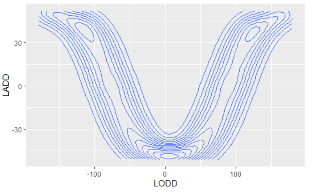
Finally, the projection of the CanSat trajectory on earth, as captured by the integrated GPS sensor, is depicted below.


We would like to thank our mentors Mr Hurley and Mr Eamonn for their support, as well as Mr Harrison and Mr Van Setten for accompanying us to the launch event.  

Our team


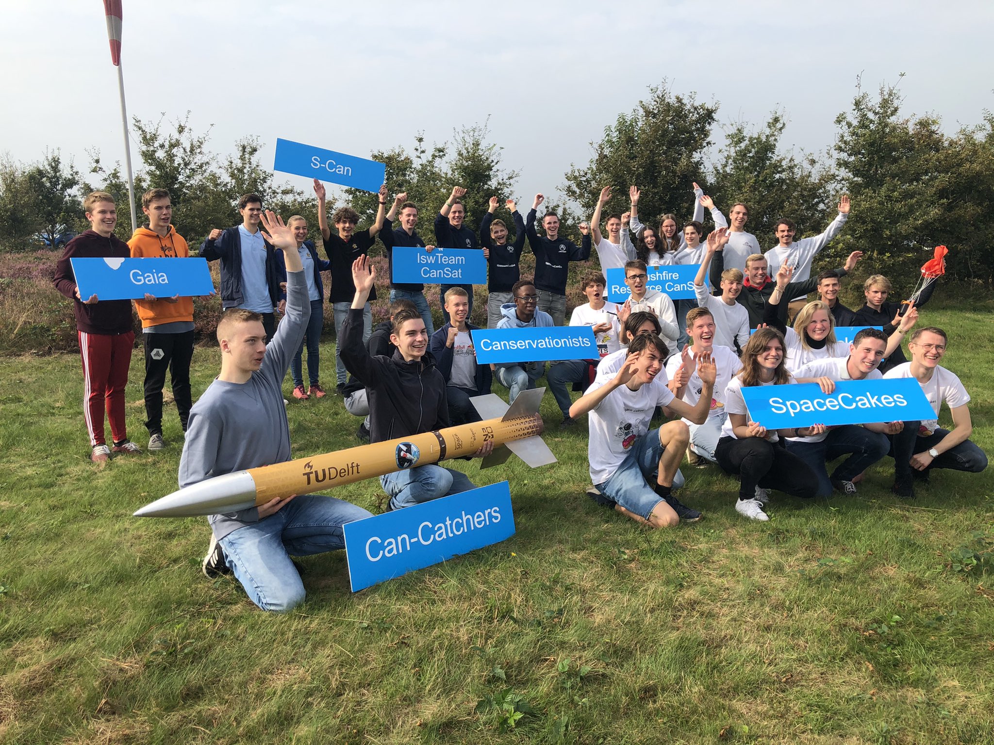
The CanSat teams that participated at the launch.


Wednesday 11 August 2021

Our Experiments at ISS (AstroPi competition) - Studying the South Atlantic Anomaly and the Van Allen Radiation Belt

In this blog post we will describe our experience from our participation to ESA AstroPi competition, the measurements we took, and our observations, and in particular regarding the so called South Atlantic Anomaly and the Van Allen Radiation Belt. 


What is AstroPi?

ESA - Astro Pi Mission Space Lab key visual

But first things first. AstroPi - Mission Space Lab, is a competition organized by the European Space Agency (ESA) in collaboration with Raspberry Pi Foundation. The aim is for teams to design and code a computer program, using the Python programming language, to be run on the International Space Station (ISS) on a Raspberry Pi. The teams have the option of focusing on life in space or life on earth. Participants have to collect data through the program, analyze them and write a report to show their findings.


Our Missions

Our team (Evaggelos Atlasis, Filippos Atlasis, Antoine Mauger) decided to focus on life in space. Our primary objective was to collect data about the magnetic field as experienced from ISS while it orbited the Earth, use the measurements to create a map of the magnetic field and compare it to the world magnetic model. We expected to observe the strongest magnetic field close to the poles and observe a decrease near the equator. 

Our secondary objective was to acquire data from the rest of the sensors (temperature, humidity, barometric pressure, acceleration, and gyroscopic measurements: roll, yaw, and pitch) in order to get a better understanding of the astronauts' life and activity inside the ISS. 


Method 

For our method, except for writing the code of the program that was going to run on the ISS, we had to carry out some actions to ensure that we could obtain and analyze our results efficiently. Firstly, we minimized the code so that we could reduce the chances of errors and improve code performance, and secondly, we saved our data results in a CSV format so it would be easier to parse them for our analysis.

After parsing the data results, we used Python's Matplotlib and the programming language R to create maps and graphs that depicted our results effectively. For our primary mission, those included a map of the measured magnetic field on the ISS trajectory and a contour map with interpolation of data. For the secondary mission, we plotted the measured variables (temperature, humidity, barometric pressure, acceleration, and gyroscopic measurements) against the runtime of our code as well as determining a rolling average for some of them to help us further with our analysis.


Results

Our program ran on the 23rd of April from around 18:46 to 21:41. 

Primary Mission: Magnetic Field Measurements

By combining the measured magnetic field  with the ISS trajectory we created a contour diagram that interpolated magnetic field strength, as shown in Figure 1. The diagram matches our expectations as the lines indicate a stronger magnetic field near the poles.  


Diagram, histogram

Description automatically generated

Figure 1: An interpolated contour map of the magnetic field measurements during the ISS trajectory


Then, we plotted the measured magnetic field along the trajectory of the ISS (Figure 2). The generated map also matches the world magnetic model and our prediction, except from the area around South America (where the colour is red, indicating a stronger measured magnetic field than the measurements in the Indian ocean where the colour is yellow). 

Figure 2: Actual measured magnetic field measurements during the ISS trajectory
 
 
By checking the world magnetic model (Figure 3), we found out that the magnetic field of the Earth around the area of the South Atlantic is weaker than the magnetic field at the same level of latitude around the Earth. 


Figure 3: World Magnetic Model 
(picture from https://ngdc.noaa.gov/geomag/WMM/data/WMM2020/WMM2020_F_BoZ_MILL.pdf)


The weaker magnetic field of the Earth at the area of the South Atlantic results in the South Atlantic Anomaly (SAA) of the Van Allen radiation belt (Figure 4).


Figure 4:  The South Atlantic Anomaly 
(picture from https://en.wikipedia.org/wiki/South_Atlantic_Anomaly)


The Van Allen radiation belt is an area of energetic charged particles which extend from an altitude of 640 to 58,000 km from the Earth's surface. The radiation is repelled by the Earth's magnetic field. In the South Atlantic area, the Van Allen radiation dips to a lower altitude as low as 200 km, because the magnetic field of the Earth is weaker at that area of the planet, resulting in the South Atlantic Anomaly.

As the ISS orbits at a height of 400 km, it passes through the Van Allen radiation belt above the SAA, experiencing an increase in the measured magnetic field from the ISS in the South Atlantic region; this increase is visible from the map in Figure 2. 

On the contrary, the SAA is not noticeable in Figure 1 as the interpolation used to produce the contours "cleaned" the anomaly.   


Secondary Mission

From our humidity measurements, there were two significant observations which can be seen in Figure 5

- There were a lot of fluctuations throughout the runtime of our code.

- The rolling average seems to significantly decrease from 19:15 to 20:00 before settling at ~31% for the rest of the runtime of our AstroPi. For the second observation, we can assume that the activity of the astronauts fell off during that time period; potentially this could be dinner time followed by some rest.

Figure 5:  Measured ISS Humidity versus time

We also observed that the temperature of the surroundings was almost identical to the CPU temperature data while reaching temperature readings of 28-29 degrees Celsius (which was 7-8 degrees Celsius higher than the actual temperature inside the ISS) - Figure 6. Thus, the temperature of the surroundings recorded by our sensor was being affected by the heat coming from the CPU and we deduced that we couldn't use our temperature data to draw a conclusion regarding the astronauts' activities in the ISS. 

Figure 6: Measured Temperature in ISS versus Time

Finally, pressure (Figure 7) and acceleration (Figure 8) data didn't show any abrupt changes in the runtime of our code (but just some fluctuations).

Figure 7: Measured Pressure in ISS versus Time

Figure 8: Measured ISS acceleration versus Time
 

Thus, we can conclude that that there was neither an O2 re-pressurization in the ISS nor an orbital acceleration which would have been apparent if they had taken place (the second conclusion is confirmed by Figure 8 where we can see that in the 23rd of April of 2021 there is no re-boost).  

 
mean height in km 
 
                                                 Figure 8: ISS height versus time
(figure from https://www.heavens-above.com/IssHeight.aspx) 
 

Conclusions

The biggest finding of our investigations was the difference in the magnetic measurements between the South Atlantic and Indian Ocean regions. After some research, we understood that this is due to the South Atlantic Anomaly (SAA) and its effect to the Van Allen radiation belt. Due to the weaker magnetic field in the area, the Van Allen radiation dips to a lower altitude. Therefore, when the ISS passes through it, the magnetic field in the region is stronger. 

From the above we understand that aerospace engineers when designing satellites that are expected to operate inside the Van Allen zone need to seriously consider its effects to their scientific measurements and operational activities, especially if spacecrafts are expected to pass through the South Atlantic anomaly area, since this can cause everything from periodic glitches to total mission failure. Indeed, the SAA has been responsible for several spacecraft failures and even dictates when astronauts can and can’t perform spacewalks. More information for the SAA and its effects on scientific missions can be found here

You can find our code here and our report here.

After the completion, we received the following nice certificate :-) We hope you enjoyed it as much as we did ;-)